7 Keyboard Shortcuts for the Filter Drop Down Menus

This post will explain 7 keyboard shortcuts for the filter drop-down menus.  This includes my new favorite shortcut, and it’s one that I think you will really like!

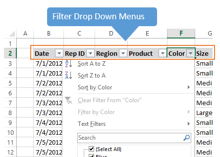
The Filter drop-down menus (formerly known as Auto Filters in Excel 2003) are an extremely useful tool for sorting and filtering your data.  When the Filters are applied you will see small drop-down icon images in the header (top) row of your data range.

These menus can be accessed with keyboard shortcuts, which makes it really fast to apply filters and sorting to different columns in your table.  So let’s take a look at these shortcuts.

#1 – Turn Filters On or Off

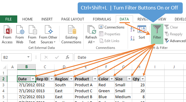
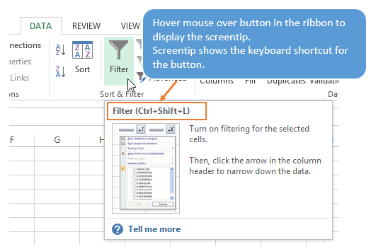
Ctrl+Shift+L is the keyboard shortcut to turn the filters on/off.  You can see this shortcut by going to the Data tab on the Ribbon and hovering over the Filter button with the mouse.  The screen tip will appear below the button and it displays the keyboard shortcut in the top line.  This works with a lot of buttons in the ribbon and is a great way to learn keyboard shortcuts.  See the image below.

To apply the drop down filters you will first need to select a cell in your data range.  If you data range contains any blank columns or rows then it is best to select the entire range of cells.
Once the data cell(s) are selected, press Ctrl+Shift+L to apply the filters.  The drop down filter menus should appear in the header row of your data, as shown in the image below.

#2 Display the Filter Drop Down Menu

Alt+Down Arrow is the keyboard shortcut to open the drop down menu.  To use this shortcut:

1. Select a cell in the header row.  The cell must contain the filter drop down icon. 
2. Press and hold the Alt key, then press the Down Arrow key on the keyboard to open the filter menu.

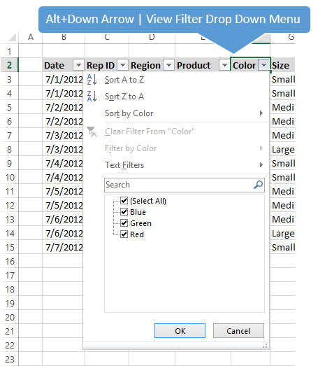
Once the drop down menu is open, there are a lot of keyboard shortcuts that apply to this menu.  These shortcuts are explained next.

#3 Underlined Letters & Arrow Keys

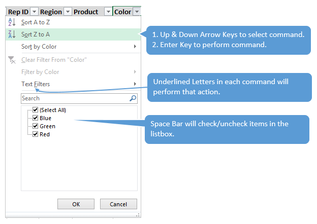
The underlined letters in the drop-down menu are the shortcut keys for each command.  For example, pressing the letter “S” on the keyboard will Sort the column A to Z.  You must first press Alt+Down Arrow to display the drop down menu.  So here are the full keyboard shortcuts for the filter drop down menu:

• Alt+Down Arrow+S – Sort A to Z
• Alt+Down Arrow+O – Sort Z to A
• Alt+Down Arrow+T – Sort by Color sub menu
• Alt+Down Arrow+I – Filter by Color sub menu
• Alt+Down Arrow+F – Text or Date Filter sub menu

#4 Check/Uncheck Filter Items

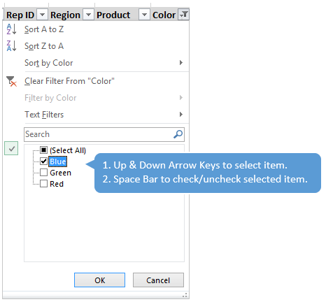
The up and down arrow keys will move through the items in the drop down menu.  You can press the Enter key to perform that action.  This requires the drop down menu to be open by first pressing Alt+Down Arrow.  See the image in #3 above for details.

Starting in Excel 2007, a list of unique items appears at the bottom of the filter drop down menu with check boxes next to each item.  You can use the up/down arrow keys to select these items in the list.  When an item is selected, pressing the space bar will check/uncheck the check box.  Then press Enter to apply the filter.

#5 Search Box – My New FAVORITE

Starting in Excel 2010 a Search box was added to the filter drop-down menu.  Excel 2011 for Mac users also get this feature.
This search box allows you to type a search and narrow down the results of the filter items in the list below it.

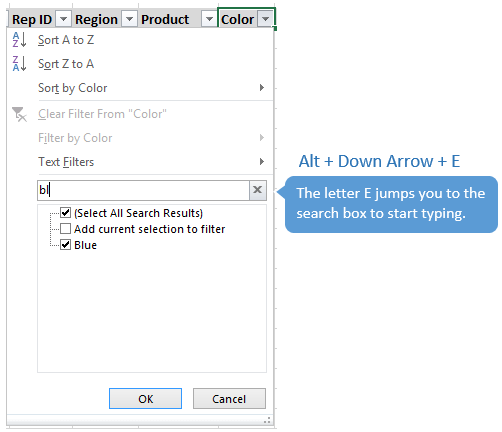
When the filter drop down menu is open, you can press the letter “E” on the keyboard to jump to the search box.  This places the cursor in the search box and you can begin typing your search.
Alt+Down+Arrow+E is the shortcut to open the filter drop down menu and jump directly to the search box.
I just learned this shortcut and it is my new favorite because it makes it so fast to type and filter exactly what you are looking for in the list.  Prior to learning this I was using the down arrow key to get to the search box.  This required me to press the down arrow key 7 times to get to the search box.  Now I can do the same thing in one step by pressing the letter “E”.  What a time saver!

#6 Clear Filters in Column

Alt+Down Arrow+C will clear the filters in the selected column.  Again, this is a combination of the Alt+Down Arrow to open the filter menu, then the letter “C” to clear the filter.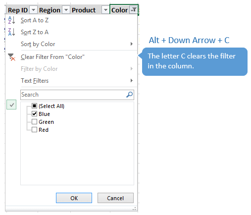

This would be the same as pressing the (Select All) checkbox in the item list.  The next shortcut will explain how to clear all the filters in all columns.

#7 Clear All Filters

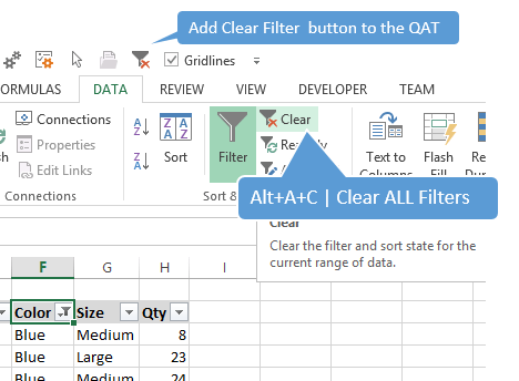
Alt+A+C is the keyboard shortcut to clear all the filters in the current filtered range.  This means that all the filters in all the columns will be cleared, and all rows of your data will be displayed.

I add the Clear Filter button to the Quick Access Toolbar (QAT) and would highly recommend that you do this.  It serves two purposes that are very helpful.

1. You can quickly press the button in the QAT to clear the filters.  If you are a mouse user this means you don’t have to navigate to the Data menu to access the button.  You can also use keyboard shortcuts to press the buttons in the QAT.  See my articles on how to setup the Quick Access Toolbar  and how to use the QAT’s keyboard shortcuts for instructions on this.
   _
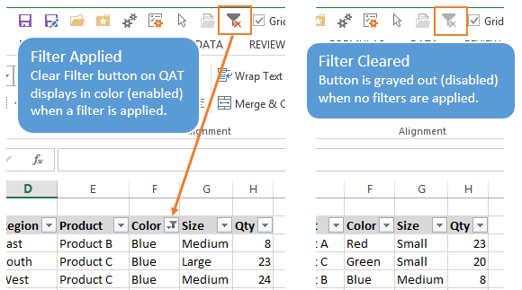
2. Use the button to visually see if any filters are applied.  This is the most important benefit to me.  If any filters are applied to the filter range, then the Clear Filter button in the QAT will show color (enabled).  If no filters are applied then the button is grayed out (disabled).  See the image below for details.
   _
   Debra Dalgleish has a great post and video with a few additional tips to Clear Excel Fitlers with a Single Click over at the Contextures blog.

#8 Filter for Blank or Non-blank Cells or Rows

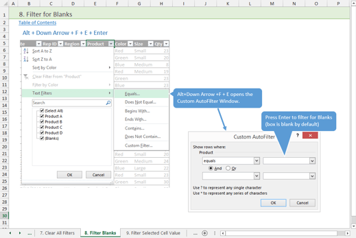
Alt+Down Arrow+F+E+Enter will filter for blanks cells in the column.

The F,E combo opens the Custom AutoFilter menu where you can type a search term.  The box is blank by default.  So if you just hit Enter when the Custom AutoFilter menu opens, the column will be filtered for blanks.
This is another one of my new favorites!  It’s much faster than unchecking the Select All box, then scrolling to the bottom of the item list.
You can also filter for Non-blanks using the shortcut Alt+Down Arrow+F+N+Enter.  This opens the Custom AutoFilter menu and sets the comparison operator to does not equal.  The criteria is blank by default, so this applies a filter for non-blank cells.  Thanks to Nilesh for leaving a comment and inspiring this one!

Bonus Tip

Typically you can only have one range filtered on a sheet at a time.  This means that if you have more than one range of data on a sheet, you can not apply the Filters menus to both ranges.
If you use the new Excel Tables feature (introduced in Excel 2007 and available for 2011 for Mac) then you can apply Filters to each table in the same worksheet.

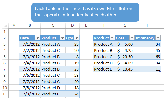
Checkout my video tutorial on Tables to learn more about all the great time saving benefits they have to offer.

Want More? – Download the Workbook

I hope you’ve learned some new tricks that will save you time when working with Filters.  In my opinion, the keyboard shortcuts are the fastest way to work with these menus.  I encourage you to practice these techniques, and also share them with a friend that might benefit.
I have also created a free workbook that contains over 25 keyboard shortcuts for the Filter Menus. The workbook is organized by topic and contains images that will help you learn the shortcuts.  It also includes a data table where you can practice the shortcuts.

Filter Drop-down Shortcuts Workbook Sample Page

Filter Drop-down Shortcuts Workbook.xlsx
Please click the link above and the Excel file that contains the shortcuts will be emailed to you immediately.